Author: Mark Whitfield

Welcome to my site! After graduating in Computing in 1990, I accepted a position as a programmer at a Runcorn based software house specialising in electronic banking software, namely sp/ARCHITECT-BANK on Tandem Computers (now HPE NonStop). This was before the internet became more prevalent and so the notion of enabling desktop access to company accounts for inter-account transfers and book keeping was still quite a cutting edge idea (and smartphones only ever hinted at in Space 1999). The company was called The Software Partnership (which was taken over by Deluxe Data in 1994). I spent 5 years in Runcorn developing code for SP/ARCHITECT for various banks like TSB, Bank of Scotland, Rabobank and Girofon (Denmark) to name but a few. I then moved onto a software house in Salford Quays for further bank facing projects. After a further 23 years in the IT industry and now a Senior IT Project Manager (both Agile and Waterfall delivery), I thought I would echo out my Career Profile in this corner of the internet for quick and easy access.

Requirements Traceability Matrix RTM & Business Analyst BA

A Requirements Traceability Matrix (RTM) is a structured project management document that links user and stakeholder requirements directly to their corresponding design elements, development deliverables, and verification test cases.

Acting as a living checklist throughout the project life cycle, its primary purpose is to ensure 100% test coverage, validate that all client requests are fulfilled, and prevent scope creep by identifying undocumented work.

The visual layout of a typical RTM template maps individual requirement rows against critical validation milestones.

🔄 Three Main Types of Traceability

The configuration of an RTM depends heavily on the direction of tracking needed for the project:

Forward Traceability: Tracks requirements forward into design, code, and test cases. It ensures the project executes every requested feature and that nothing gets left behind.
Backward (Backward-Looking) Traceability: Traces test cases and final deliverables back to the original requirement. It checks for scope creep, confirming that no extra, unauthorized features were added.
Bidirectional Traceability: Combines both approaches. It links requirements from origin to destination and vice versa, providing clear visibility during change management or troubleshooting.

📋 Structured Breakdown of RTM Content

A standard RTM is formatted as a multidimensional table. Below is the foundational structure, broken down into its logical data components:

1. Core Requirement Parameters

Requirement ID: A distinct alphanumeric identifier (e.g., REQ-001, BRD-102) for quick cross-referencing.
Requirement Type: Classifies the item (e.g., Business, Functional, Technical, UI, Security, or Regulatory Compliance).
Requirement Description: A concise textual explanation defining exactly what the feature or system must achieve.
Source/Origin: The document, stakeholder, client request, or meeting minutes where the requirement originated.
Priority Level: The urgency ranking of the item, usually categorized as High, Medium, or Low (or via MoSCoW ranking).

2. Design and Development Artifacts

Functional Specification ID: Links the requirement to the specific section of the functional design document.
Technical Design/Architecture Module: Points to the code packages, database tables, or system architectural components implementing the requirement.

3. Verification & Validation (Testing) Data

Test Case ID: The unique ID of the specific test cases designed to validate the feature (e.g., TC-101, TC-102).
Test Case Description/Objective: A snapshot of what the test case actually checks.
User Acceptance Testing (UAT) ID: Specific ID linking to end-user validation scenarios.

4. Execution & Quality Control Tracking

Test Execution Status: The real-time health indicator of the testing suite (e.g., Passed, Failed, Blocked, Not Run).
Defect/Bug ID: If a test fails, this column logs the active issue tracker ID (e.g., Jira ticket BUG-404) linked to the breakdown.
Current Deployment Status: Defines the project readiness stage (e.g., In Progress, Dev, QA, Production).

💡 Core Benefits of Maintaining an RTM

Prevents Missed Features: Verifies that every business requirement translates into clean code and valid testing cycles before software deployment.
Streamlines Change Management: If a client alters a feature, developers can quickly scan the RTM row to see exactly which code modules and test scripts need updates.
Simplifies Compliance Audits: Serves as regulatory proof in safety-critical landscapes (like medical devices or automotive software) that every target function passed validation.

Requirements Traceability Matrix RTM & Business Analyst BA

Bluetooth Overview and Detailed Chronological Timeline

Bluetooth is a universal, short-range wireless communication standard that enables electronic devices to exchange data and audio over ultra-high frequency (UHF) radio waves (operating between 2.402 GHz and 2.480 GHz). It forms localized, temporary networks known as piconets to seamlessly bridge data gaps without the clutter of physical wires or cables.

To combat signal congestion in the crowded 2.4 GHz band—which it shares with Wi-Fi and microwaves—Bluetooth uses a technique called Adaptive Frequency Hopping (AFH), rapidly switching between 79 or 40 channels up to 1,600 times per second to maintain a stable, secure connection.

Named by Intel engineer Jim Kardach after the 10th-century Scandinavian King Harald “Bluetooth” Gormsson—who famously united warring Danish tribes into a single kingdom—the technology was built to similarly unify incompatible PC, cellular, and digital device ecosystems. The iconic Bluetooth logo is a direct nod to this heritage, fusing the ancient Norse runes ᚼ (Hagall) and ᛒ (Bjarkan) representing King Harald’s initials.

Bluetooth Overview and Detailed Chronological Timeline

🏛️ Era 1: Pre-Commercialization & Foundation (1989–1998)

Before becoming an open global standard, Bluetooth began as a proprietary corporate feasibility project aimed at liberating electronics from restrictive RS-232 data cables.

1989: Nils Rydbeck (CTO of Ericsson Mobile) and inventor Johan Ullman initiate a “short-link” radio technology project designed to develop comfortable wireless headsets.
1994: Jaap Haartsen and Sven Mattisson are tasked by Ericsson leadership to formally design the hardware infrastructure in Lund, Sweden. They focus on low-power, low-cost radio architectures.
1997: The engineering team achieves a functional, workable link layer solution. Intel’s Jim Kardach proposes the temporary codename “Bluetooth”.
1998: Recognizing a global framework requires cross-industry alignment, Ericsson joins forces with IBM, Intel, Nokia, and Toshiba to found the Bluetooth Special Interest Group (SIG) to establish an open, license-free standard.

📱 Era 2: The Classic Bluetooth Era (1999–2009)

The first commercial implementation focused heavily on replacing peripheral wires. However, early builds struggled with device-role conflicts, high power consumption, and severe data limitations.

1999 (v1.0 & v1.0b): The Bluetooth SIG publishes the official Bluetooth 1.0 specification. It is heavily plagued by interoperability issues and mandatory hardware address exposure, creating distinct privacy gaps.
2001 (v1.1): Standardized globally under the IEEE 802.15.1 banner. Fixes version 1.0 connection bugs, supports point-to-multipoint slave connections, and introduces unencrypted channel support. The Sony Ericsson T36 debuts as the first commercial phone with integrated Bluetooth.
2003 (v1.2): Introduces Adaptive Frequency Hopping (AFH) to stop Wi-Fi network interference. Adds Extended Synchronous Connections (eSCO) to rescue voice audio quality by allowing packet retransmissions.
2004 (v2.0 + EDR): Unleashes Enhanced Data Rate (EDR). Maximum throughput leaps from a nominal 721 kbps to 3 Mbps, greatly reducing power draw through shorter transmission cycles.
2007 (v2.1 + EDR): Introduces Secure Simple Pairing (SSP). This eliminates complex PIN-code handshakes, improving device security while seamlessly supporting Near Field Communication (NFC) proximity pairings.
2009 (v3.0 + HS): Debuts High Speed (HS) architecture. It uses a clever dual-radio configuration where Bluetooth creates the initial handshake, but offloads large media payloads to an internal 802.11 Wi-Fi link for speeds up to 24 Mbps.

🔋 Era 3: The Bluetooth Low Energy (BLE) & IoT Era (2010–2015)

Prior versions consumed too much power for miniature electronic applications. This era redefined the standard, establishing an entirely separate protocol tier optimized to run on tiny coin-cell batteries for the burgeoning Internet of Things (IoT) market.

2010 (v4.0): The pivotal launch of Bluetooth Low Energy (BLE) (branded initially as Bluetooth Smart). Devices can remain asleep until data bursts happen, drastically dropping baseline energy consumption.
2013 (v4.1): Engineers adjust software layers to prevent direct frequency collision with 4G LTE bands. Devices can now act as both an independent hub and peripheral sensor simultaneously.
2014 (v4.2): Designed entirely for smart home architecture, this update adds support for IPv6 and 6LoWPAN. This allows smart sensors to connect directly to the internet without intermediary mobile gateways.

🌐 Era 4: High-Performance & High-Precision Mesh Era (2016–Present)

Modern iterations have fundamentally transformed the technology from a basic local data-link pipe into a highly robust, secure mesh network and precision spatial positioning framework.

2016 (v5.0): Doubles BLE transmission speeds to 2 Mbps and quadruples operational range up to 240 metres. It optimizes performance for large-scale smart homes and multi-room layouts.
2019 (v5.1): Introduces Direction Finding via Angle of Arrival (AoA) and Angle of Departure (AoD) antennae arrays. Devices achieve hyper-local indoor positioning down to centimeter-level accuracy.
2020 (v5.2): Unveils LE Audio running over the highly efficient LC3 Codec. It introduces Auracast, which enables a single source device to stream high-fidelity audio to an infinite number of nearby headphones or hearing aids.
2021 (v5.3): Adds connection subrating to reduce communication switching latencies. Improves peripheral device power optimization and encryption control keys.
2023 (v5.4): Adds Periodic Advertising with Responses (PAwR) alongside Encrypted Advertising Data (EAD). This allows two-way secure mass communication, tailored specifically for thousands of commercial electronic shelf labels.
2024 (v6.0): Incorporates groundbreaking Channel Sounding technology. It employs phase-based time-of-flight measurements to provide centimeter-level distance awareness, creating incredibly secure digital car and home keys that prevent relay signal tracking attacks.

Bluetooth Overview and Detailed Chronological Timeline

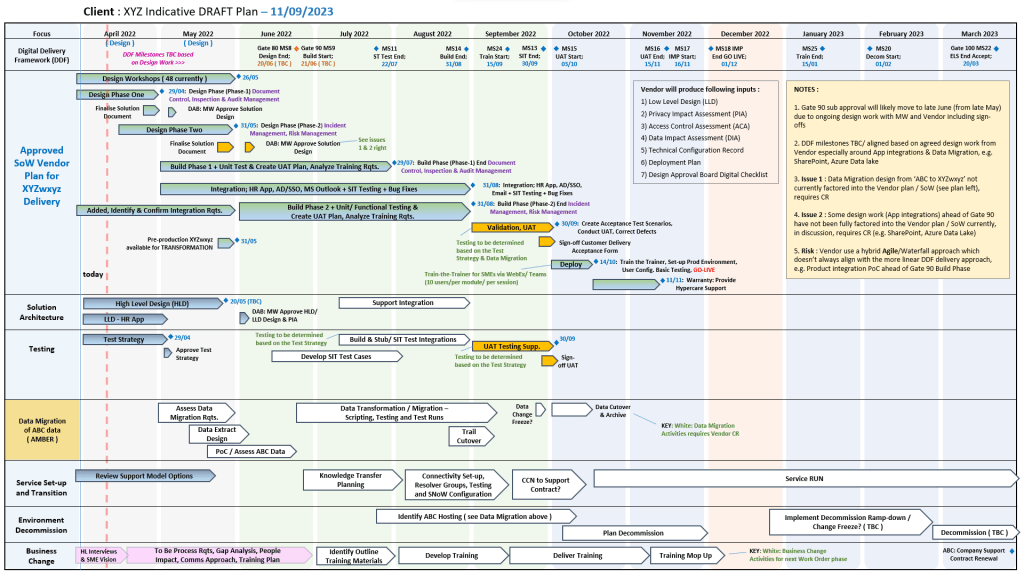
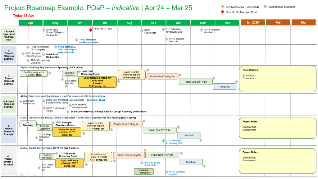
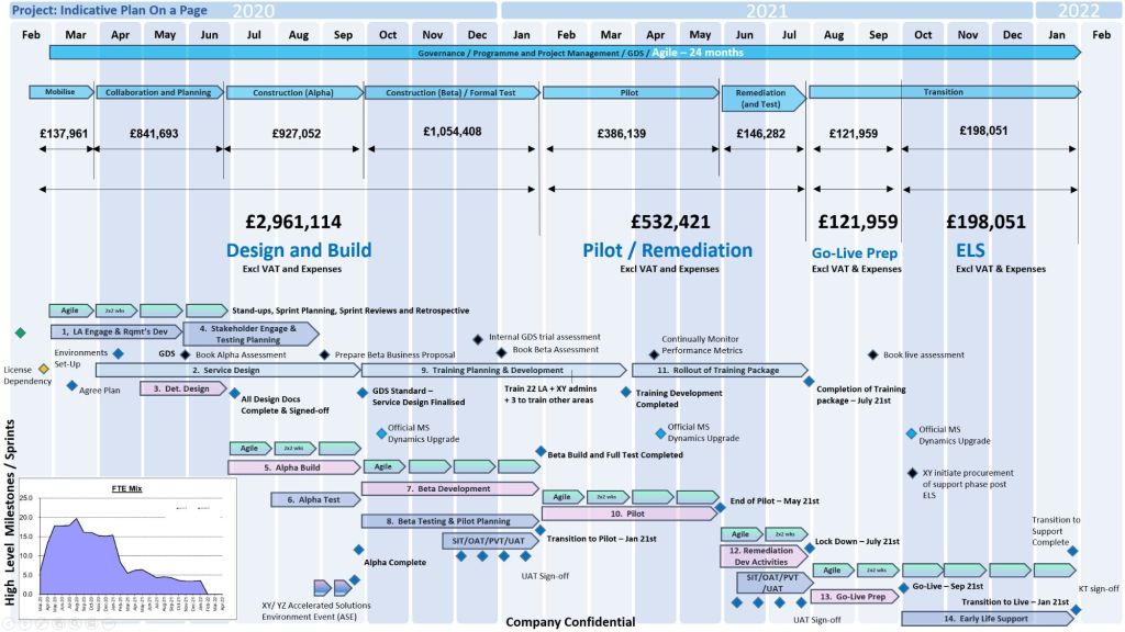
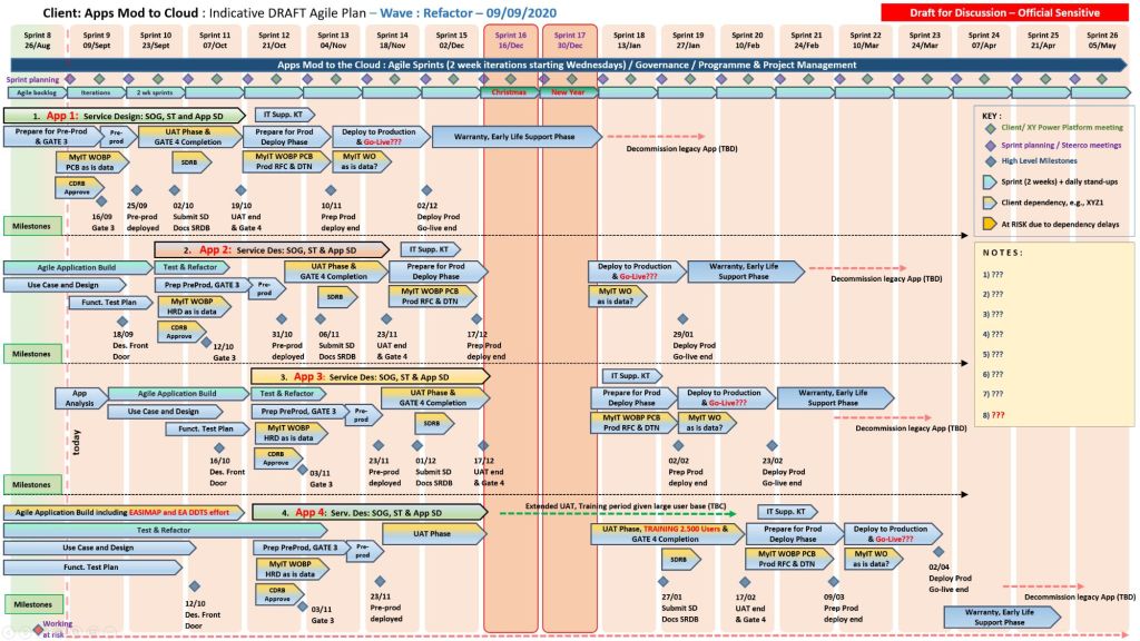
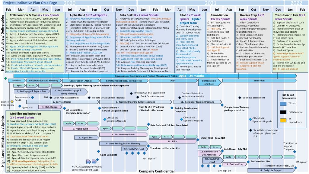
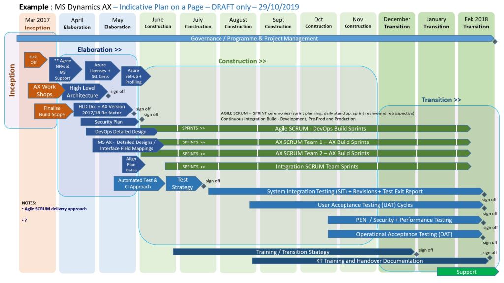
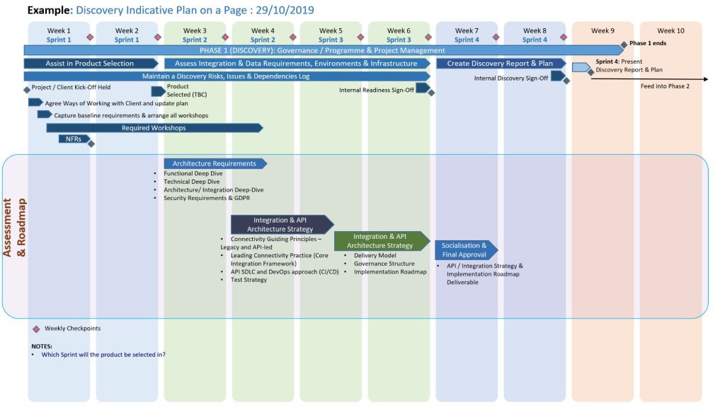
Agile Delivery Journey from Requirements to Release

HPE NonStop Pathway is a transaction processing & application server environment (TS/MP)

HPE NonStop Pathway is a premier transaction processing and application server environment (TS/MP) that powers mission-critical Online Transaction Processing (OLTP). It handles critical application services—such as fault tolerance, load balancing, memory management, and process scheduling—automatically, allowing developers to focus strictly on business logic.

Detailed Timeline Breakdown

The history and evolution of the Tandem NonStop platform and its Pathway environment span decades of architectural transformations and corporate ownership, categorized by distinct hardware and software eras:

1. The Tandem Era (1974–1997)

1974: Tandem Computers Inc. is founded by Jimmy Treybig to build the first fault-tolerant commercial hardware.
1976: The first Tandem NonStop system (NSI) is launched. Early apps had to be manually coded for fault tolerance.
1981: NonStop II is released, bringing 32-bit addressing.
1983: The Transaction Monitoring Facility (TMF) is introduced. Together with the launch of the Pathway transaction management software, the need for programmers to write manual fault-tolerance logic into their code is officially eliminated.
1986: Tandem releases the EXT as an entry-level system, followed by the VLX.
1991: Tandem introduces the Cyclone/R and initiates a massive architectural shift away from proprietary stack machines towards MIPS RISC processors.
1997: Compaq acquires Tandem Computers, placing the NonStop product line under its umbrella.

2. The Compaq & Early HP Era (1997–2014)

2001–2002: Hewlett-Packard (HP) merges with Compaq. The platform is rebranded as HP NonStop.
2005: The HP Integrity NonStop (TNS/E) series is introduced, migrating the fault-tolerant platform to Intel Itanium microprocessors. Pathway continues to be the main driver for high-volume banking and telecom applications.
2011: Further hardware advancements lead to the release of HP Integrity NonStop BladeSystems.

3. The Modern HPE Era (2015–Present)

2015: Hewlett-Packard splits, and the NonStop environment transitions to Hewlett Packard Enterprise (HPE).
2015/2016: Introduction of NonStop X (TNS/X) systems, marking the platform’s migration to standard Intel x86-64 processors and adopting InfiniBand interconnects. Pathway capabilities are updated to span dynamic server classes across multiple systems (Pathway Domains).
Present: HPE continues to modernize the NonStop architecture, integrating the platform with HPE GreenLake for consumption-based models and providing native support for modern DevOps tools and hybrid cloud deployments.

HPE NonStop Tandem EMS Subsystem Overview and Chronological Timeline

In the HPE NonStop ecosystem, EMS (Event Management Service) is the core software subsystem responsible for collecting, formatting, filtering, logging, and routing system and application event messages. It provides fault-tolerant monitoring by gathering data from EMS collectors and selectively delivering alerts to consoles, log files, or automated management applications.

EMS events as viewed in Console, Reflex 80:20 event viewer (ITL) — EMS event detail as viewed in Console, **Reflex 80:20 event viewer (ITL)**

EMS event view configuration window in Console — EMS event view configuration window in **Console**

The evolution and detailed historical timeline of NonStop EMS events and architecture is broken down by era below:

1. The Tandem Guardian Era (Late 1970s – 1980s)

Focus: Foundation of Fault-Tolerant Event Logging

1976: Tandem releases the original Tandem/16 (NonStop I) system. Early event handling was primarily a rudimentary terminal console logging process.
1978: System administrators struggled with message scaling as clusters and terminal networks expanded. Tandem began developing structured event tracking, paving the way for standardized subsystem messages.
1980s: Introduction of early message formatting. Event messages 1 through 511 were reserved for unformatted, raw console events. The Event Management Service (EMS) was gradually formalized to centralize scattered terminal messages.

2. The D-Series & TMF Era (1990s)

Focus: Distributed Management & The Birth of Modern EMS

1991: Tandem releases the Cyclone/R (CLX/R) and later the Himalaya K-series using MIPS processors.
1993: The publication of the seminal EMS Reference Summaries standardized EMS APIs and SPI (System Programming Interface). Event IDs were structured into standardized subsystems (e.g., negative-numbered kernel messages).
1995: The NonStop Kernel introduced Open System Services (OSS), natively integrating Unix-like event logs into the Guardian architecture.
1997: Compaq acquires Tandem Computers. EMS underwent significant rewrites to interface with remote servers and client networks. The S-Series was launched utilizing ServerNet fabric, introducing advanced, distributed event collectors and distributors.

3. The Compaq Transition & HP Integration (2000s)

Focus: Web-Based Management and Automation

2000 – 2003: Legacy ViewPoint tools were expanded. The emergence of GUI interfaces and DSM/PM (Distributed Systems Management/Performance Monitor) allowed operators to browse and filter EMS logs on alternate/primary event files.
2003 – 2005: The transition to Web ViewPoint commenced, turning text-based EMS event logs into interactive, web-based graphical operations interfaces.
2006 – 2009: With HP fully in charge after merging with Compaq, EMS event viewing was modernized through TSM (Tandem/HP Systems Management) and the Open System Management (OSM) Event Viewer.

4. The Modern HPE Era (2010s – 2026)

Focus: Cloud Integration, Virtualization, & Real-Time Analytics

2015 – 2017: The platform is rebranded as HPE NonStop as the architecture migrates to x86 processors. EMS systems are upgraded to handle large datasets, feeding complex event processing (CEP) and SNMP trap frameworks for modern data centers.
2018 – 2023: HPE integrates NonStop systems with HPE GreenLake. EMS event logging is modernized with API-driven integrations, allowing system events to be consumed by off-platform enterprise loggers, Splunk, and cloud-management consoles.
2024 – 2026: EMS events operate in highly virtualized and hybrid cloud (x86 and Virtual NonStop) environments. Event management heavily relies on modern distributed systems where EMS distributors push logs seamlessly into centralized IT monitoring suites and continuous availability dashboards.

To look up specific system-generated event codes or statuses from any era, consult the legacy ⁠HP NonStop Operator Messages Manual or the broader ⁠HPE Nonstop Compute documentation portal.

Story Mapping in Agile Scrum

Story Mapping in Agile and Scrum is a visual technique that organizes user stories along a chronological user journey. It helps teams see the big picture, avoid flat, disconnected backlogs, and collaborate on planning iterative releases that consistently deliver user value.

How a Story Map is Structured

A story map is a two-dimensional grid—often built with sticky notes on a whiteboard or via software like ⁠Miro or ⁠Visual Paradigm. It breaks work down into three levels of hierarchy:

Horizontal Axis (The Spine): Arranges the customer journey chronologically.
- Activities: The broadest goals a user wants to achieve (e.g., “Checkout”).
- Steps: The specific tasks required to complete the activity (e.g., “Enter Shipping Info,” “Pay”).
Vertical Axis (Details & Priority): Stacks beneath each step are the detailed user stories, epics, or features. They are organized by priority, with the most critical or highly sophisticated tasks at the top.

The Benefits of Story Mapping

Teams use this technique—popularized by Jeff Patton—to achieve several core Agile goals:

Prevents “Flat Backlog” Blindness: Gives stakeholders and developers a birds-eye view of how the entire application or feature fits together.
Defines the MVP: Allows teams to draw horizontal “release lines” across the map. The items sitting above this line form the barebones “walking skeleton” or Minimum Viable Product (MVP).
Aids Sprint Planning: Helps the Product Owner pull well-sequenced, context-aware stories directly into sprint backlogs.
Fosters Collaboration: Moves the team away from siloed requirement docs and toward collaborative conversations around actual user behavior.

MoSCoW Requirements Prioritization Method

The MoSCoW method is a popular requirements prioritization technique used in project management and software development to help stakeholders reach a common understanding on the importance of deliverables. It categorizes tasks into Must, Should, Could, and Won’t have.

The MoSCoW Categories

Must Have: Non-negotiable requirements that are critical for success, compliance, or safety. Without these, the project is considered a failure and cannot be deployed.
Should Have: High-priority, important features that add significant value but are not strictly vital for immediate delivery. These are generally included if time permits, or they may have a manual workaround.
Could Have: Desirable, “nice-to-have” features that are small and easy to implement. These improve user experience but can be deferred or dropped without impacting the project’s overall success.
Won’t Have (or Won’t Have this time): Features that have been mutually agreed upon as out-of-scope for the current release or timeframe. They are deliberately excluded to prevent scope creep, though they may be added to the backlog for future cycles.

Why and When to Use It

Resource Management: It helps maximize limited time, budget, and resources by focusing effort on the features that provide the most immediate ROI.
Stakeholder Alignment: It acts as a negotiation tool, forcing stakeholders to agree on what is genuinely critical versus what is purely desirable.
Agile Environments: It is a foundational practice in Agile frameworks like DSDM, where teams adhere to fixed deadlines (timeboxes) and adjust the project scope instead.

Best Practices for Implementation

The 60-20-20 Rule: A common best practice is to ensure that Must Haves consume no more than 60% of the team’s total effort. Roughly 20% should be allocated to Should Haves, and 20% reserved for Could Haves to act as contingency room.
Challenge Assumptions: When classifying a requirement as a Must, ask: “What happens if we don’t do this? Can we still deploy the product?” If the project can still function—even awkwardly—it is likely a Should or Could.
Continuous Review: Priorities aren’t static. Re-evaluate your MoSCoW list at the end of every sprint or development cycle, as a Could Have from a previous phase might be upgraded or permanently discarded.

MoSCoW Requirements Prioritization Method

Frameworks for Business Analysts BAs

Frameworks for BA Business Analysts BAs — Frameworks for Business Analysts BAs

Share this:

Share this:

Share this:

Share this:

Share this:

Share this:

Share this:

Share this: